Recommendation Systems

Intro

Recommendation systems are typically characterized by the existence of:

Users
Items

The goal is to predict and suggest items to users that they are likely to be interested in, based on their past behavior, preferences, and interactions with the system. These systems of have users and items in the millions or even hundreds of millions. Some common use cases of recommendation systems are:

Personalizing e-commerce experiences by recommending products based on browsing and purchasing history.
Suggesting movies, TV shows, and music on streaming platforms tailored to user preferences and viewing history.
Curating content such as articles, blogs, and news on digital platforms according to user interests and reading habits.
Enhancing social media engagement by recommending friends, pages, and content based on interactions and network connections.
Targeting online advertisements to users based on their demographics, online behavior, and preferences.
Matching job seekers with relevant job listings on recruiting platforms using their skills, experiences, and career objectives.
Connecting individuals on dating apps with potential matches by leveraging profile information and preference settings.
Recommending travel destinations, accommodations, and packages on travel sites based on past bookings and search history.
Suggesting courses and learning materials on educational platforms by analyzing user interests and previous learning activities.
Recommending games and apps in digital stores, considering user's past downloads and activity patterns.

A User-Item interaction matrix, where rows are users and columns are items, is often the starting point. Since the number of items used, rated, etc. by users is typically small relative to the number of items, this User-Item matrix is sparse.

Matrix Factorization

Matrix factorization is one way to learn user-item similarities. Matrix Factorization in recommendation systems decomposes a user-item interaction matrix, \(R\), into two smaller matrices, \(U\) and \(M\), representing latent factors of users and items such that \(R \approx U \times M^T\). This facilitates the prediction of user preferences for previously uninteracted items.

For example, the user-item interaction matrix \(R\) is given by:

\[ R = \begin{pmatrix} 5 & 3 & ? & 1 \\ 4 & ? & ? & 1 \\ 1 & 1 & ? & 5 \end{pmatrix} \]

Here, "?" indicates that the user has not rated the movie. Our goal is to predict these missing ratings. We initialize the matrices \(U\) (user features matrix) and \(M\) (movie features matrix) into \(m\ x\ d\) and \(n\ x\ d\) matrices, where \(m\) is the number of users, \(n\) is the number of items (movies in this case) and \(d\) is the embedding size of the latent factors, as follows:

\[ U = \begin{pmatrix} 0.1 & 0.2 \\ 0.3 & 0.4 \\ 0.5 & 0.6 \end{pmatrix}, \quad M = \begin{pmatrix} 0.7 & 0.8 \\ 0.9 & 1.0 \\ 1.1 & 1.2 \\ 1.3 & 1.4 \end{pmatrix} \]

Through an optimization process, such as stochastic gradient descent (SGD) or Alternating Least Squares (ALS) where the loss function could be Mean Squared Error (MSE) loss, we iteratively adjust \(U\) and \(M\) to minimize the difference between \(R\) and \(U \times M^\top\) for the known ratings. After convergence, we might end up with updated matrices:

\[ U' = \begin{pmatrix} 0.5 & 0.6 \\ 0.7 & 0.8 \\ 0.9 & 1.0 \end{pmatrix}, \quad M' = \begin{pmatrix} 1.5 & 1.6 \\ 1.7 & 1.8 \\ 1.9 & 2.0 \\ 2.1 & 2.2 \end{pmatrix} \]

To predict the missing rating for the first user on the third movie, we calculate the dot product of the corresponding user vector and movie vector:

\[\text{Predicted Rating for User 1, Movie 3} = \begin{pmatrix} 0.5 & 0.6 \end{pmatrix} \cdot \begin{pmatrix} 1.9 \\ 2.0 \end{pmatrix} = 0.5 \times 1.9 + 0.6 \times 2.0 = 1.85 \]

Two-Tower Neural Network

Architecture

Another way to learn user-item similarities is to use a "Two-Tower" neural network. The idea here is that the network has two parallel inputs: one for user data and one for item data. Each 'tower' computes an embedding. The embeddings are then compared via a similarity metric such as inner product. This architecture is shown below in figure 1:

Figure 1: Example graph: Two Tower Neural Network

Training:

The model is trained in a supervised way, where labels are determined from user actions. Labels often are based on the following:

Item watched, ordered, etc.
User rating of item
User 'liked' item

In cases where the interaction is binary, like watching a video, the label can be weighted based on other criteria to give more label resolution. For example, videos could be weighted by the percentage viewed. Using features like watch time tend to perform better than features like 'click-through', as the latter is prone to promoting clickbait.

The vector of user features is often called the query and the vector of item features is often called the candidate. The input features capture things like the user (in the case of query) as well as additional potentially useful context (date/time, device, etc.). We'll call the query \(x\) and the item \(y\). So one way we can train is to have training examples of triplets \((x_i, y_i, r_i)\) where \(r_i\) is the weight mentioned above (also called the reward). For example, \(r\) could be 1 or 0 depending on whether a user bought an item, a 1-5 rating, etc.

The goal is to find items that match user features well. This can be seen as a classification problem over all the items. For example, assume there are \(M\) items. We could send all items through the item tower, dot product the resulting embeddings with the query embedding, resulting in \(M\) scores. We could then take the softmax and train using cross entropy loss.

So, for a given query x the probability of picking item y from M items, where \(\theta\) contains the two tower model parameters and s(x, y) is the dot product of embedded vectors x and y after going through their respective towers, is given by

\[ P(y \mid x; \theta) = \frac{e^{s(x, y)}}{\sum_{j \in [M]} e^{s(x, y_j)}} \tag{1}\label{1}\]

By incorporating the weights (rewards) we can compute a loss over the batch, where T is the batch size:

\[ L_T(\theta) = -\frac{1}{T} \sum_{i \in [T]} r_i \cdot \log(P(y_i \mid x_i; \theta)) \tag{2}\label{2}\]

One major problem is that often \(M\) is too large to be feasibly calculated. To work around this, we can sample a subset of items, \(B\), from \(M\) and use this as an estimate of all items. This is known as the sampled softmax:

\[ P_B(y_i | x_i; \theta) = \frac{e^{s(x_i, y_i)}}{\sum_{j \in [B]} e^{s(x_i, y_j)}} \tag{3}\label{3}\]

If \(y_i\) was interacted with by \(x_i\) then it is a positive example, otherwise it's a negative example. However, this introduces another problem: Since users interact with a small percent of all items, this sampling is essentially from a power-law distribution so that popular items are over-represented as negatives. To fix this we adjust the score \(s(x_i, y_i)\) by subtracting from it the sampling probability of item j:

\[ s_c(x_i, y_j) = s(x_i, y_j) - \log(p_j) \tag{4}\label{4}\]

This essentially upweights the scores of items that are seen infrequently. There are various methods to approximate \(p_j\). A common one is streaming frequency estimation, where we have an up to date exponentially weighted average of the number of batches since the last instance of item \(y_i\) was seen. The inverse of this then gives us \(p_j\).

By replacing \(s(.)\) with \(s_c(.)\) in equation \(\ref{3}\), giving us \(P_B^c\), we get the batch loss sampled over the batch as follows:

\[ L_B(\theta) = -\frac{1}{B} \sum_{i \in [B]} r_i \cdot \log(P_B^c(y_i | x_i; \theta)) \tag{5}\label{5}\]

We now have an architecture and loss function and can train the model.

Alternative Loss (Noise Contrastive Estimation)

In the previous section the loss function was computed as follows: Get a batch of samples, compute the sampled softmax, and use the cross entropy loss with along with the item weights to get a batch loss. Another similar loss function, noise contrastive estimation (NCE) loss, is also commonly used. Like the sampled softmax it uses negative sampling, but rather than having a softmax over the batch it treats each example as a binary classification problem.

For example, we compute the sigmoid of every user-item pair and then sum these up to get a batch loss. If the user didn't interact with the item (or the rating was very low, etc.) then the sigmoid should output close to 0 for this pair. On the other hand, if the user-item interaction is high, then the sigmoid should be close to 1. Thus, the loss for a training example with 1 positive user-item interaction and \(k\) negative samples is:

\[ \text{Loss} = -\log \sigma(x \cdot y_{pos}) - \sum_{k_{\text{neg}} \in \mathcal{N}} \log \sigma(-x \cdot y_{k_{\text{neg}}}) \tag{6}\label{6}\]

Where \( \mathcal{N} \) represents the set of \(k\) negative samples drawn from the noise distribution. Note that typically \(k\) ranges from about 5 to 20. The loss over a batch is thus:

\[ \text{BatchLoss} = \frac{1}{B} \sum_{i=1}^{B} \left( -\log \sigma(x_i \cdot y_{pos_{i}}) - \sum_{k_{\text{neg}} \in \mathcal{N}} \log \sigma(-x_i \cdot y_{k_{\text{neg}, i}}) \right) \tag{7}\label{7}\]

Inference

With the two towers of the model each trained we can do inference. In order to do this in real time, the item embeddings have already been computed by passing all items through the item tower. These vectors are then stored for fast approximate nearest neighbor (ANN) similarity search using tools like Faiss or ScaNN. When a new query comes in it is passed through the query tower to get an embedding vector. This embedding vector is then passed to the ANN algorithm to retrieve the top k most similar items.

Recommendation Considerations/Techniques

This section will outline a variety of techniques and tips for architecting, training, and improving recommendation systems.

Unsupervised Embeddings

Item embeddings can be learned in a way similar to how word embeddings can be learned by predicting neighboring words (i.e. target words from context words as in continuous bag of words, or context words from target word as in skip-gram). For example, a playlist of movies or songs can be used in a model to try to predict neighboring items in the sequence.

Features other than just "items" can also have learned embeddings. For example, a user's list of search items can be useful feature embeddings. Each search item would be tokenized and then embedded. One approach is to simply sum all the embeddings in the search history list to create a single dense embedding feature. These search would then be learned as part of the overall network training. In this scenario recommendations could be based off search history before any videos are even watched.

Avoiding Staleness

Having the age of the item as a feature (for example 0 if it's brand new) can help the model prioritize new items, which is often desired.

Surrogate Task is Important

When creating recommendation engines, other tasks ("surrogate" tasks) are typically solved and those solutions are transferred to the recommendation problem. Predicting ratings is different than providing recommendations, but it's assumed ratings are indicative of good recommendations. Always consider whether assumptions from the surrogate task are accurate, and be clever with new surrogate tasks!

Consider video recommendations based on a user's watch history. The training data is a sequence of watched videos. One training strategy could be to guess videos watched based on neighboring videos in the sequence. For example, given video 4 and 6 learn to recommend video 5. In practice this strategy of performs poorly because users have an ordering preference. Videos are often watched sequentially. Episode 5 is watched before episode 6.

To address this, the future video should be predicted based on previous watch history, rather than learning videos based on surrounding watched videos. This is an example of how subtleties of the learning task can greatly affect real world performance.

Avoiding User Over-representation

It's common for highly active users to have an outsized effect in recommendations. One solution is to generate the same number of training examples per user. For example, if User A has rated 1,000 items and user B has rated 10 items, only select 10 items per user when training. This helps the opinion of few but active users swaying all recommendations too much.

Churn (Sequential Requests)

When dealing with multiple iterations of recommendations, previous recommendations should be considered. For example, if the previous batch of items sent as recommendations were not interacted with, those items should be down-weighted when determined the next batch of items to be recommended. Clearly we don't want to keep sending items the user is not interested in.

Common Architectures

In the beginning of this post we discussed the Two Tower architecture, where each tower learns user and item embeddings respectively. Different problems require different architectures, and even the same problem may benefit from an architecture other than the Two Tower. In this section a variety of other architectures will be briefly discussed.

Deep Candidate Generation

The following architecture is from a YouTube recommendation engine:

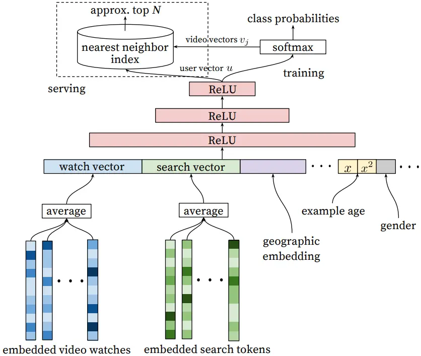
Figure 2: Deep Candidate Generate (source)

It uses an embedding, similar to continuous bag of words, to combine various length features into single vector embeddings. Video embeddings in a playlist are added together two get one embedding. The same is done with search queries from search history.

These embeddings, along with other features such as geographic location, user age, etc. are all concatenated to create the input feature. This feature is then propagated through the network to get class probabilities over the items. Sampled softmax is used with cross-entropy loss for training. During recommendation serving the user vector is compared to item vectors using approximate nearest neighbor search (e.g. Faiss).