Introduction to Transformers
This tutorial will cover the fundamentals of the transformer architecture.
Basic Building Blocks
At the highest level, the transformer architecture is made up of two separate pieces: an encoder and a decoder. Both the encoder and decoder are made up of N repeating blocks. In the original Transformer paper the authors' set N = 6. In the example image below N = 4. The encoder takes the inputs and encodes a representation of them. This encoded representation is then passed to the decoder, along with additional inputs, to generate a prediction.

For natural language processing (NLP), the input to the encoder is a tensor of shape [batch size, maximum input sequence length]. Maximum input sequence length is the longest sentence that the transformer could encounter. The output from the decoder is shape [batch size, maximum output sequence length, vocabulary length]. Vocabulary length is the amount of words your model has in its dictionary. For example, a popular early transformer Bidirectional Encoder Representations (BERT), has a vocab length of about 30k words.
Each block of the decoder receives as input the output from the last block of the encoder. During training, the decoder also receives the target sentence, shifted one word to the right, as input. During inference (when the target is not available), the decoder instead receives the output from the previous step. This means the decoder is called multiple times, extending the sequence by one word each time until the-end-of-sequence token <EOS> is output from the decoder. This type of model, where the previously generated output is consumed as an additional input in the next step, is known as an auto-regressive model. This process is depicted in Figure 1 above.
The main advantage of the architecture we've discussed so far, compared to the previous architectures for handling sequences such as Recurrent Neural Networks (RNNs), is parallelization. In an RNN, the encoding process is sequential, where one input produces a hidden state, that hidden state plus the next input produces the next hidden state, etc. With the Transformer architecture, the encoding process is done in a single parallel step with the entire input. But transformers have additional benefits over RNNs. Next we'll take a more detailed look at the layers that make up a transformer.
Layers in Detail
Figure 2 below shows the layers of a transformer in detail. We'll now discuss each layer in detail, starting from the bottom and moving up.

Sources:
The input to the encoder is a tensor of integers, where each integer corresponds to a word in the input sentence. Since the network needs to work with numbers and not strings, we can't input the sentence, "I like dogs". Thus, sentences are first converted to lists of words, a process called tokenization. So tokenizing, "I like dogs" would result in the list ["I", "like", "dogs"].
Next, each token is mapped to an integer is. This is called numericalization. If our dictionary has 10k words, then maybe "I" is word 103, "like" is 1294, and "dogs" is 3099. These are just arbitrary numbers chosen for this example, but the point is that we are mapping a word to a number.
Additionally, Since the entire sequence is input altogether (i.e. not one word at a time as in an RNN), the shape needs to be consistent yet accommodate sequences of varying length. This is done by having a maximum length input, and padding the sequence until it has a specific length. Most models have a maximum length of 512 or 1024 tokens.
For our example, let's say the maximum sequence length is 10 and the padding token is 0. Using the word to number mappings stated above, the input to the embedding layer would be [[103, 1294, 3099, 0, 0, 0, 0, 0, 0, 0]]. This is a shape of (1, 10): batch size of 1, sequence length of 10. Notice how the padding token 0 was used to pad the sequence length to 10, providing a consistently sized input.
Embedding Layer:
The embedding layer is a mapping of a tokenized word to its representation in vector space. For example, if each word is represented by 512 dimensions, our embedding layer weights will be a matrix of shape [dictionary size, 512]. Each row corresponds to the vector representation of a specific token. If our source is "I like dogs", tokenized to integers 103, 1294, and 3099, then the embedding process will extract rows 103, 1294, and 3099 from the embedding matrix. The values of these vector representations are learned during training.
This layer is essentially identical to a linear layer, where each of our inputs is a one-hot vector. However, for computational efficiency reasons it's computed using an index lookup based on the token rather than the matrix multiplication of a long one-hot vector and a weight matrix.
The output shape of this layer is (batch size, max sequence length, embedding dimension).
Positional Encoding:
Since the input is provided all at once in parallel, rather than sequentially one word at a time like in an RNN, there needs to be some way for the model to know about the positions of the words. This is accomplished through positional encodings. The number of positional encodings will be the same as the maximum input sequence length (i.e. there will be one positional encoding for every word of the input, just how there is a word embedding for every word in the input). These positional encodings are vector representations, with the same dimension as the word embedding vectors, so that each positional encoding can be added to its corresponding word embedding.
These positional encodings can either be learned or fixed. A learned positional encoding is simply a vector with d learnable weights, where d is the dimensionality if the encoding (e.g. 512).
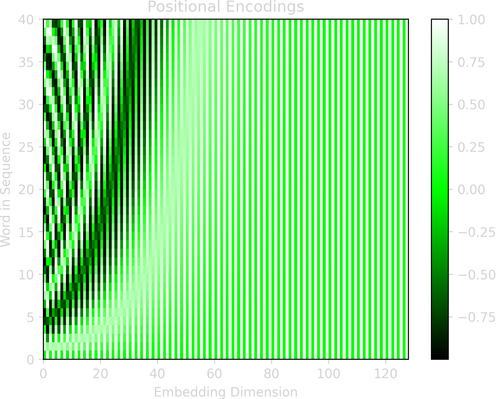
The authors of the original transformer paper, however, use a fixed positional encoding. The equation below is how the value for each component of the positional encoding is calculated:
\[ PE_{p, 2i} = sin(p / 10000^{2i/d}) \] \[ PE_{p, 2i+1} = cos(p / 10000^{2i/d}) \]
\(PE_{p, i}\) is the positional encoding value of the \(ith\) component of the encoding vector for the word at position \(p\) in the sentence. The figure below shows these encoding values for a sequence with 40 words and an encoding vector of 128.
These fixed sinusoidal encodings give the same performance as learned encodings, but have the advantage that they may allow the model to extend better to longer sentences than were seen during training. Additionally, the sinusoidal function assists the model in learning relative positions.
Let's quickly recap what we've done so far:
- Converted the input sequence of words to tokens
- Mapped each token to an embedding vector of learnable weights
- Mapped each position in the sequence to a positional encoding using the sinusoidal equation above
- Summed each token embedding with its positional embedding
Next, we'll take a look at attention mechanisms, which is the heart of the transformer architecture (and hence why the paper was titled Attention Is All You Need).
Attention Layer Overview:
The general idea behind attention is to put extra focus on certain inputs (or features). For example, if the input is a sentence, attention is useful to focus on some words more than others. The attention mechanism uses two components to focus attention:
- The inherent saliency a word has (e.g. "fire" may draw more attention that "the")
- The relevance of the word to the task at hand (e.g. performing a language translation task and trying to locate the verb in a sentence after the subject has been translated)
Imagine you're driving around looking for an ice cream shop. A bright, flashy store sign will draw more attention than a bland sign. This is comparable to the first attention component. Signs with "Ice Cream" will also draw more attention than signs for other shops. This is synonymous to the second attention component.
The first type of attention can simply be computed using vanilla fully connected layers. Weights corresponding to inputs or features that are of particular importance become larger during the training process.
The second component of attention can be learned as follows: Imagine there exists a vector representation of some concept. Take for example, the representation of a part of speech (noun, verb, etc.). Now, imagine we have the sentence "She runs fast", where a part of speech is mapped to each word in the sentence (pronoun: She, verb: runs, adjective: fast). If we want the model to focus on the verb, we would like to look up the words in the sentence by the key "verb" and see what we get.
However, in reality our representations of these keys (verb, adjective, etc.) are not discrete values, and instead are embedded in vector representations. So the model can't perform the mapping in the way a literal dictionary lookup works (e.g. sentence['verb']).
Instead, the model can find which vector representation of the part of speech is most similar to what it's looking for by using a cosine similarity (i.e. the dot product). So, if the model is trying to find the word that is a verb, it takes its vector representation of a verb, and computes the dot-product of this vector representation with the part of speech representation of every word in the sentence. The dot-product with the highest value is the word presumed to most likely be the verb.
In transformer terminology, the concept that we are trying to find is the query. We compare the query to each of the keys, and then weight the value that each key is mapped to by how similar the key is to the query.
Attention Layer Calculation:
Now that the attention layer has been covered conceptually, let's look at the details of the calculation.
The following calculations will be done for each encoder. The input to each in encoder is matrix \(X\), which has shape [nkeys, nembed]. For the first encoder \(X\) is the embedded words. For all subsequent encoders \(X\) is the output from the previous encoder.
\(Q\) is the Query matrix. It has shape [nqueries, dkeys], where nqueries is the number of queries and dkeys is the dimensionality of each key. So \(Q\) is a matrix where each row is a query vector, and there's one row for each query.
\(Q\) is calculated by doing a matrix multiplication of \(X\) by the query weights matrix, \(W^Q\) (which has shape [nembed, dkeys]): \[ Q = XW^Q \] Since there will be a query for each key, nkeys = nqueries.
\(K\) is the Key matrix. It has shape [nkeys, dkeys], where nkeys is the number of keys and dkeys is the dimensionality of each key. So \(K\) is a matrix where each row is a key vector, and there's one row for each key.
\(K\) is calculated by doing a matrix multiplication of \(X\) with the key weights matrix, \(W^K\) (which has shape [nembed, dkeys]): \[ K = XW^K \]
\(V\) is the Value matrix. It has shape [nkeys, dvalues], where nkeys is the number of keys and dvalues is the dimensionality of value vector. So \(V\) is a matrix where each row is a value vector and there's one row for each key.
\(V\) is calculated by doing a matrix multiplication of \(X\) with the value weights matrix, \(W^V\) (which has shape [nembed, dvalues]): \[ V = XW^V \]
Now that \(Q\), \(K\), and \(V\) have been calculated, they can be used to calculate attention.
First, take the dot product of each query vector with each key vector. This will produce positive values for key vectors that are very similar to query vectors, and negative values for key values that are very different than the query vectors: \[ QK^\top \] This results in a matrix of [nqueries, nkeys], meaning we have compared every query vector with every key vector. These are sometimes referred to as similarity scores. The idea is to use these values to scale the value vectors in \(V\): \[ QK^\top V \] Producing a matrix of [nqueries, nvalues], which is a weighted sum of the value vectors for each query.
However, there is one issue with the calculation above: We want to reduce the magnitude of value vectors whose keys did not match well with the query vectors. But the dot product for a poor match between a query and key vector will produce a large negative value rather than a value close to 0.
To resolve this, the softmax is computed prior to multiplying by the \(V\). Additionally, since the magnitude of the dot product grows with the number of elements, a scaling factor \(1/\sqrt{d_k}\) is used. This helps prevent the softmax values from saturating leading to small gradients. The entire attention calculation is shown below:
\( \textrm{Attention}(Q, K, V) \) \( = \textrm{softmax}\left(\dfrac{QK^\top}{\sqrt{d_k}}\right)V \)
In words, here's what this equation is saying:
- Take the dot product of every query with every key. This gives a scalar for every query, key combination.
- Divide all of these scalars by \(\sqrt{d_k}\)
- Take the softmax of these values over the key dimension. That is, for a given query \(q\), take the softmax over all the resulting \(q\cdot k_i\) dot products for \(i\) in 1...nkeys. These are the similarity scores.
- For a given query, multiply each similarity score by its corresponding value vector. Then sum all these scaled vectors. Doing this for all queries results in a single vector for each query, where each vector is a sum of all the weighted value vectors for that query.
Multi-Head Attention:
In order to make the model more expressive and able to learn more representations, multiple attention mechanisms are used per encoder. This is accomplished by doing the exact calculation described in the previous section h times, using different weights each time. The results of each of these h attention calculations are then concatenated together and multiplied by a weight matrix \(W^O\). In the original transformer paper h=8 (this is referred to as the number of heads.
Let's look at an example of how this is computed for 2 heads. First we calculate the first attention head using \(W_1^Q\), \(W_1^K\), \(W_1^V\):
\( \textrm{Attention}_1(Q_1, K_1, V_1) \) \( = \textrm{softmax}\left(\dfrac{Q_1K_1^\top}{\sqrt{d_k}}\right)V_1 \)
Then we calculate the second head in the exact same way, except we use \(W_2^Q\), \(W_2^K\), \(W_2^V\):
\( \textrm{Attention}_2(Q_2, K_2, V_2) \) \( = \textrm{softmax}\left(\dfrac{Q_2K_2^\top}{\sqrt{d_k}}\right)V_2 \)
This give two matrices, Attention1 and Attention2, each with dimensions [nqueries, dvalues]. They are then concatenated along the dvalues dimensions, resulting in a single matrix of size [nqueries, 2 * dvalues].
Last, this concatenated attention matrix is multiplied by a weight matrix \(W^O\). This gives an output size from the multi-head attention layer equal to the input size. The shape of \(W^O\) is [h * dvalues, dkeys], where h is the number of heads (h=2 in this example, h=8 in the original paper).
Position-wise Feed-Forward Layer:
The output of the concatenated multi-head attention layer (referred to as \(Z\) in the equation below) goes into a position-wise feed-forward layer (FFN). This layer is simply two fully connected layers with a ReLU activation in between:
\( \textrm{FFN}(Z) \) \( = \textrm{ReLU}(ZW_1+b_1)W_2+b_2 \)
The input and output to the FFN has a dimensionality of 512, and the inner layer has a dimensionality of 2048. Thus, the shape of \(W_1\) is [512, 2048] and the shape of \(W_2\) is [2048, 512].
Skip Connections and Normalization:
The last components of Figure 2 remaining to discuss are the skip connections (aka the residual connections) and the layer normalization.
The skip connections occur around the self-attention layers and the feed-forward layers. The dimensionality of the input to the self-attention is the same as the output from the self-attention, so the input and output are summed.
Similarly, the input to the feed-forward layer is the same dimensionality as the output, so the input and output are also summed.
This resulting sum is then passed through layer normalization.
A visual of the skip connection followed by layer normalization is shown below. \(X\) is the input to the multi-head attention layer (or feed-forward layer), and \(Z\) is the output from the multi-head attention layer (or feed-forward layer). Add & norm is a sum of \(X\) and \(Z\) follow by layer normalization.
Layer normalization is calculated by first getting the mean and standard deviation over each embedding vector. In the example above that would be a mean and standard deviation for each row. Then the mean is subtracted from its corresponding embedding vector and the result is divided by the corresponding standard deviation.
And that's it for the details of how transformers are constructed!
The original transformer architecture was created for translation, but there have since been many variations specialized for other tasks. In this last section, we will briefly look at modifications to the original transformer model, and see how the encoder and decoder can be used either independently or together to solve problems other than translation.
Transformer Models:
Encoder Models use just the encoder portion of the transformer. They're often used for tasks that need to understand the entire sentence, such as question answering, sentence classification, and named entity recognition (e.g. detecting things such as person names, company names, location names, etc. and classifying them).
Examples of encoder models are
- BERT: A transformer model designed to pre-train deep bidirectional representations
- DistilBERT: A distilled version of BERT: smaller, faster, cheaper and lighter
- RoBERTa: A Robustly Optimized BERT Pretraining Approach
- ELECTRA: A pre-training approach using Text Encoders as Discriminators Rather Than Generators
Decoder Models use just the decoder and are often used for tasks like generating sentences. This is words are generated one at a time, and as a result the attention layers only have access to the words prior to the current one. This kind of sequential generation is known as an auto-regressive model, and are often used for things like sentence generation.
Examples of decoder models are
- GPT: Generative Pre-Training
- GPT-2: An even larger GPT
- RoBERTa: A Robustly Optimized BERT Pretraining Approach
- Transformer-XL: An Attentive Language Model Beyond a Fixed-Length Context
Encoder-Decoder Models, which is what the original transformer architecture is, is used for tasks where the input and output are both sequences (often referred to as seq-to-seq models. Common seq-to-seq tasks include translation, text summarization, or generating new sentences given input sentences.
Examples of encoder-decoder models are